As a warning, this is more of a brief technical report on the xG values you’ll see in my shot maps this season. It will get quite boring and overly technical. If you’re wanting to read the usual fun articles about Stoke then check back in a day or two for something much more exciting!

Given the vast range of incredibly useful and free data available through sites like FBref.com, Whoscored.com, Infogol and SofaScore among others, you might think there’d be no need to develop your own tools and models for a low-readership blog about as niche a topic as Stoke City FC.

But, as you may well know from my work here, I can’t leave well-enough alone.

Location data in football can be relatively easy to come by in the form of pre-made images and maps. Wyscout is a (relatively) cheap platform that provides these for shots, passes, and other events during games. Whoscored and similar sites provide things like heat maps, pass maps, and other location plots for free, too.

But, finding the raw data can be either a very long or a very expensive process. Access to raw location data via subscriptions, even for one league, can cost several thousand pounds a year.

As a result, you’ll notice that most of my location data last season was through pre-made plots from WyScout.

This season, however, Potterlytics is finally evolving! Having found a method to reliably and cheaply get this data, you can look forward to shot maps, pass maps, heat maps, and so many other maps that I might end up contacting Jay Foreman for a spot on Map Men.

There is, however, one issue. This new, exciting data, doesn’t include with it a measure of the most accepted of advanced metrics, Expected Goals (xG). If you can’t remember how xG works, or just want to remind yourself, check out the previous article on how it works here: xG – A Stoke City Explainer!

There was a possibility that I could cross-match my data with data from sites that do provide xG, such as FBref.com, or the Wyscout platform, but this became impossible to automate. Shots with one provider are not necessarily shots with other providers, for example, and the small differences in shot data on a game-by-game basis made it incredibly time-consuming to ensure each shot was matched with its correct xG counterpart.

It became clear, either I spend the rest of my days matching every shot in one dataset to another dataset by hand, or I come up with my own model.

Luckily, I have experience with predictive modelling in my day job (check out some astronomy we did on predicting stellar ages here! https://ras.ac.uk/news-and-press/news/getting-foot-cosmic-age-ladder-using-machine-learning-estimate-stellar-ages), and so I decided to try and have a go myself.

So, with big apologies to those of you not interested in the minutiae of statistical models who were just looking for a nice Stoke article, here is a brief technical report on how I developed an approximating xG model to suit my data visualisations.

xPect the un-xPected

The goals then was as follows:

• To generate a predictive model of xG that can closely replicate realistic probabilities with a less- comprehensive dataset.
• Determine uncertainties on this model and evaluate its prediction capabilities.

Using a training dataset of ~140’000 shots from the EFL Championship (18/19 – 22/23 inclusive) and the Premier League (20/21 – 22/23 inclusive), I aimed to train an artificial neural network (ANN) to predict goal probability from the data I had available.

The dataset provided includes the most obvious, useful information required for such a model, such as x and y coordinates of shots, the body part the shot was taken with, whether it was from open play or a set piece, and calculating the method of assisting the shot (i.e. cross, through ball, counter, cut-back), was simple and has been well explained by others.

Firstly, values for the distance to the centre of goal (r) and the angle to the nearest post (theta) were calculated and replaced ‘x’ and ‘y’ in the training dataset. Additionally, a factor of ‘1/r’ was added.

Finally, the area in which I think helped make the biggest difference to this model, the ‘Big Chance’ metric.

Generally, the phrase ‘Big Chance’ from a data provider can be meaningless. With the data I have used, via Opta, it is defined as ‘A situation where a player should reasonably be expected to score’. This usually involves setting an arbitrary xG value, above which a chance is considered a ‘Big Chance’.

As my model is attempting to approximate more complex xG models like Opta Statsperform’s, the inclusion of ‘Big Chance’ as a feature of my model is a big help. It allows considerations which are not possible with the data I have, such as a goalkeeper out of position, a 1v1, or even the opposite side of the coin in a very close shot surrounded by players, to be taken into account as an average by the model.

For example, two shots, both with the right foot from 18 yards out, both assisted in the same way and functionally exactly the same shot. In one of them, the goalkeeper has been rounded and the player has an open net, in the other, there are 5 defenders and a goalkeeper blocking the path to goal. The first is defined as a big chance, the second isn’t. The inclusion of ‘Big Chance’ therefore means that my model can differentiate these shots, despite not having access to high-level positioning data.

So, with a total of 15 metrics, and a validation set of 10% of the original shots, the ANN model was trained as close to best-fit as possible, 5 times and each iteration saved.

Results

The model predictions (taken from the mean xG prediction of the 5 models) was tested on two datasets from the EFL Cup (21/22 and 22/23).

These produced positive results in the ROC curves, as shown below.

But, that’s a very boring way to check viability, and I need to be more certain that the values in shot maps won’t be ridiculous or incredibly off-the-mark.

So, let’s check via a much more fun method, comparing shot maps to leading providers!

First off, we have one of Stoke’s newest signings, Wesley.

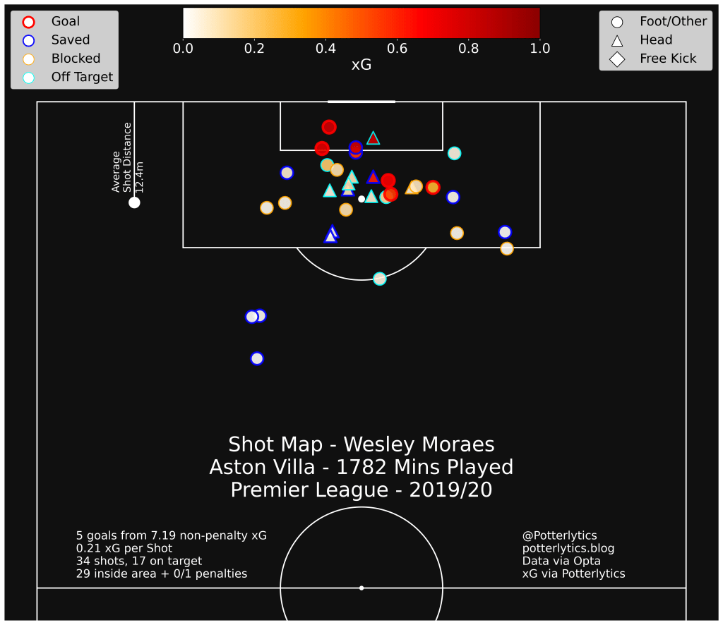
Our model is giving a total non-penalty xG of 7.19, which is worryingly far from FBref’s 5.5 npxG for this season. However, we do see a much closer agreement with Infogol’s npxG for Wesley’s season of 7.18, so I am content with the result in this regard, and content that a variation of 20% in xG is possible even between professional models!

Taking a look at the distribution of estimates across matches, we see that there’s a lot of similarity, bar a big discrepancy on one particular match day.

This corresponds to one particular match vs. Norwich, where Wesley bagged 2 goals, and missed a penalty.

Looking specifically at that match, we see the reasoning behind this discrepancy, with a large increase in xG values in my model for the higher quality chances. His first goal, a right footed finish turned into the goal with the goalkeeper bearing down, was given 0.35xG by FBref, but 0.67 by our model. This is a common theme for high-xG chances, where my model does not take into account whether it is a first time shot, the angle of the incoming pass, and the details of the advancing keeper, who was very close to Wesley.

A similar effect is seen in the rebound to his missed penalty, given 0.43xG by FBref, but 0.55xG by my model, as the keeper is within 1 yard of Wesley, and the ball is off the ground. Both of these cannot be taken account of in my model.

However, even though the mean model estimate is slightly off, there is a significant increase in the uncertainty predicted to reflect this. Both shots have a ~20% uncertainty in their xG value, as the model takes into account the range of xG values possible for these shots.

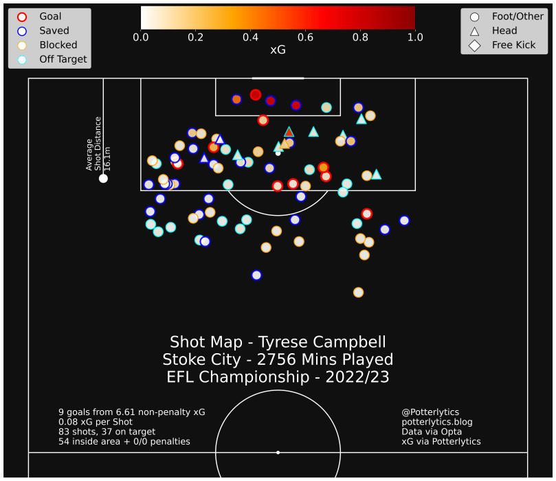
Across many other players tested, this is a common issue. For example, Tyrese Campbell’s 1st goal against Sunderland, where he slots home into an open net, is given an xG of 0.22 by my model, compared with 0.81xG by the FBref Opta model, which has access to player positions.

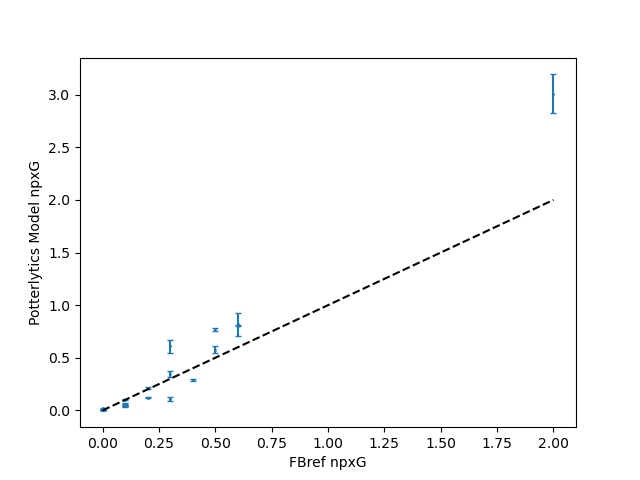
Further testing with other data (the same process with all clubs in the 17/18 Premier League season and further testing on Stoke players) shows similar results. The model tends to slightly under-predict some of the lower Opta xG chances, and over predict a few of the highest Opta xG big chances, but overall, the mean ratio of Potterlytics model match xG to Opta match xG is 1.06 ± 0.2.

If I wasn’t using this for a niche Stoke City blog, I’d show a much more in depth analysis of the models, and compare exact xG values to each of the major stats provider models. But I hope there’s at least enough evidence here for you to understand what this model does, what my xG values will be, and where the accuracies/inaccuracies are.

Conclusion

Given the original aim of the model, I’m confident that the xG values predicted provide a reasonable approximation of the more in-depth models, with appropriate uncertainties.

Looking at the principles behind the use of xG, i.e. to measure and present the ‘value’ of a given chance, I find that for my main use of these xG values, shot maps presented on the blog/Twitter/etc., the model provides suitable values that can represent this chance value.

There are more questions on the specific values given for total xG of players, and current testing is determining whether to use these xG values from the model, or to import ‘total’ values from other sources.

Honestly, if you read that and you were expecting a Stoke story, I’m so sorry.

But there we go, now I’ve explained why my xG values may differ from others you see online!

Thanks to any and all readers, and please feel free to comment and follow on Twitter at @potterlytics.

Should you wish to donate to help with the running costs of the site, and the data subscriptions we use, please feel free to visit our donations page here. Any and all help is very much appreciated!

George