You see it everywhere in football nowadays, it’s even grown to the point where Sky Sports show it on their post-match stats.

We now appear to be at a point where not only is eXpected Goals (xG) assumed to be common knowledge, it’s also something that its assumed everyone fully understands. But for a lot of people, xG is just a term that suddenly appeared and isn’t necessarily well-understood.

Considering this, I thought a good way to start off the blog here at Potterlytics would be to go through a little xPlainer (I’m sorry) of expected goals, told through the lens of Tyrese Campbell and two beautiful Stoke City goals from recent seasons.

The Basics

So let’s start by looking at the basic concept behind xG.

Football is a very low scoring game, with a high proportion of randomness to the results. It’s much easier for a lower-quality team to eek out a win through a bit of luck in football than in, say, basketball, where games finish with much higher scores.

This means that in football, the final score is generally a poor metric by which to measure the quality of a team’s performance, or to understand the major themes within a match.

As an example, you could say ‘well Stoke had 14 shots and Preston only had 3’ to show that Stoke were the better side, but on further inspection it could be the case that Stoke tried 14 Charlie Adam-esque shots from the halfway line in the last 10 minutes, and Preston had 3 shots from 5 yards out. This is the point where we’d say ‘they had the better chances’.

The best way to consider xG is that it gives you a number that quantifies just how good a chance is. Taking into account historical data, namely thousands of shots from previous seasons, an xG model tells you just how often the average player can be expected to score from a given chance.

There is no such thing as a perfect metric for the quality of a performance, but xG helps at least compare the quality of chances created.

‘How can you score 0.47 goals? What a load of ****’

xG values are usually quoted in terms of the probability of a goal being scored from zero to one. 0 xG would indicate that it’s impossible to score the chance, and 1 xG would indicate that it’s impossible to miss.

If a chance has an xG of 0.47 from a given model, that means that in that model’s historical data, a goal was scored from this type of chance 47% of the time, i.e. for every 100 of these chances, there were 47 goals.

Interestingly, it’s usually the case that xG is much lower than you’d expect, for lots of chances. xG can never be 1, as even a half-yard tap in is missed very occasionally. Let’s give a few examples and then take a look at a very fun Stoke City goal.

‘How’s he missed that?’

Take, for example, a penalty. Before you read on, think carefully and have a guess at how often you’d expect an average penalty taker to score. 90% of the time? Surprisingly it’s not that high! A penalty is in fact (using Wyscout models) 0.76xG, meaning only 76% of penalties are scored.

Extra points if you assumed lower than 0.76 because of Stoke’s record.

We can take a look below at the xG model that takes into account only the location of the shot, to see what kind of values we can expect:

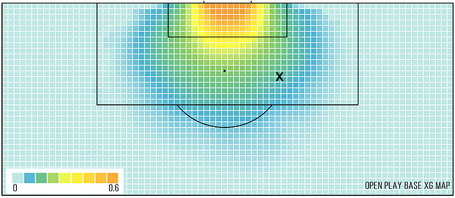
Now better models will take into account much more than just the location of the shot. Let’s use Tyrese Campbell’s goal vs Preston, from 22/23, as an example:

Unleash Tyrese

In the 2-0 away win at Preston North End, Tyrese Campbell scored the second goal with a placed shot from just inside the box. On our map above, the location is marked with an ‘x’. We see that this gives us an xG value of around 0.15, meaning a shot from this location is scored about 15% of the time according to the model.

If we look at Infogol’s model value, we see that they assign a probability of 0.12 xG to this chance.

Wyscout on the other hand, assign it a value of 0.07 xG, and FBref.com go even lower to 0.03 xG.

Where’s that difference coming from?

Well, aside from models using different datasets, which will include slightly different shots, and models themselves learning from the data differently, the major difference here is what information is included when we define a type of shot.

Looking at our first model from the map above, we see that in Campbell’s shot, he’s about 14 yards out, to the right of the goal, and that’s all the information our model has! From this, we can say only that a shot from this area results in a goal about 15% of the time.

Now, better and more rounded models can add in more info. For example, the 3 other models take into account information such as angle to the goal, how the shot was assisted (e.g. cross or through ball), and the body part with which it was taken (strong/weak foot or header).

In addition to this, many of the models will include even more infortmation. Opta data (used by FBref.com, and many professional football teams/leagues) takes into account the positioning of defenders, the status of the goalkeeper (is he set or in motion?), and the height at which the shot is struck.

We can see very simply how this affects the xG value. Our FBref value of 0.03 xG was much lower than the others, due to the pressure Campbell is under. Two defenders directly in front of him, and a set goalkeeper waiting for the shot.

The Return of the Messiah

Now we can further see this difference by comparing the Preston goal with Campbell’s first goal after his injury layoff, vs Peterborough in November 2021. He receives the ball from a pass by a teammate, and takes a shot from a similar position.

However, this time, there are two obvious differences.

Firstly, Campbell takes the shot with his weak foot, slightly decreasing the chance of scoring. More importantly, however, he has a clear view to goal, with only some pressure to his left, from a defender he has just dribbled past.

The combination of these extra differences for two chances in a similar position increases the FBref xG from 0.03 xG to 0.25 xG.

Hopefully this provides a nice intro and explainer for those who are interested in Stoke, and didn’t previously understand what xG was used for and how it was developed. Any and all comments are appreciated!

This is the first of many posts on this blog, and the aim is to contribute between once a fortnight and once a week some form of longer piece here. Alongside that, we have regular brief threads on Twitter at @potterlytics.

Should you wish to donate to help with the running costs of the site, and the data subscriptions we use, please feel free to visit our donations page here. Any and all help is very much appreciated!

George